Tutorial: from an orientation map to a textured polycrystal¶
An orientation map (EBSD) gives the grains of a section and the orientation of the crystal of each. This tutorial reads one, finds its grains and its texture, computes the stiffness of its polycrystal, pulls it into the plastic regime where its lattices turn, follows them to a large strain, and gives the texture of the map to a polycrystal of space. Each step meets a number known in advance: the mean disorientation of crystals at random, the bulk modulus of cubic crystals, the fibres of a stretched polycrystal.
The map is the one that comes with morphoGen: a section of a polycrystal of nickel as an acquisition would give it, 64 by 48 points every half micrometre, a part of its grains near the cube orientation. With a measured map only its path changes. The snippets follow each other in one session and take about twenty seconds in all, most of it the two plastic computations.
1. The map and its grains¶
An .ang file (EDAX/TSL) or a .ctf file (Oxford Instruments/HKL) is read with the
points that were not indexed, the phases and their symmetries:
import numpy as np

import morphogen as mg
from morphogen import texture
from morphogen.io import ebsd

measured = ebsd.read_ebsd(ebsd.example_map())  # or the path of a file: "my_map.ang"
print(measured.shape, measured.step)  # (48, 64) (0.5, 0.5): rows, columns; micrometres
print(round(100 * measured.indexed.mean(), 1))  # 88.0 % of the points were indexed
The orientations are brought into the axes of the image of the map — the first to the
right, the second upwards, the third towards the viewer —, which are those of the
polycrystals made of it. A .ctf file gives them so; an .ang file gives them in axes
turned about the normal, by an angle that depends on a setting of the acquisition
(read_ebsd(path, setting=1), 1 to 4: its first axis points down the image with the
usual one). A map read with the wrong setting has the right grains and the wrong
texture: theory, §92.
Two neighbouring points belong to one grain when their disorientation — the smallest angle between their lattices, their symmetries taken into account — is below a threshold. The grains are the connected sets of such points; the smallest are given to their neighbours, as are the points that were not indexed:
grains = measured.grains(threshold=5.0, min_size=5)  # degrees; points
print(grains.count)  # 56
print(round(grains.diameters.mean(), 2))  # 3.95 um: the discs of the areas of the grains
print(round(grains.spread.mean(), 2))  # 0.36 degree: the scatter inside the grains
Each grain has the mean orientation of its points. The map in the colours of the direction of each crystal along the normal (red: [001], green: [011], blue: [111]), with the boundaries of its grains:
from morphogen.viz import figures

fig = figures.ipf_map_figure(measured, grains=grains)
fig.savefig("texture_map.png")
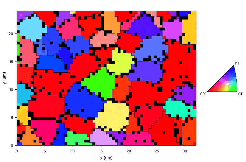
The red grains have a cube axis along the normal: the cube component of this texture.
2. Its texture¶
A pole figure shows where the normals of a family of planes point, for all the crystals together. Its density is in multiples of that of crystals at random: one everywhere without a texture. The grains count by their areas:
families = ((1, 0, 0), (1, 1, 0), (1, 1, 1))
poles = [texture.pole_figure(grains.orientations, hkl, weights=grains.areas) for hkl in families]
print([round(p.maximum, 1) for p in poles])  # [5.7, 3.6, 4.6] times random
near_cube = texture.disorientation(grains.orientations, np.zeros(3)) < 15.0
print(round(grains.areas[near_cube].sum() / grains.areas.sum(), 2))  # 0.4 of the area
fig = figures.pole_figures_figure(poles)
fig.savefig("texture_poles.png")
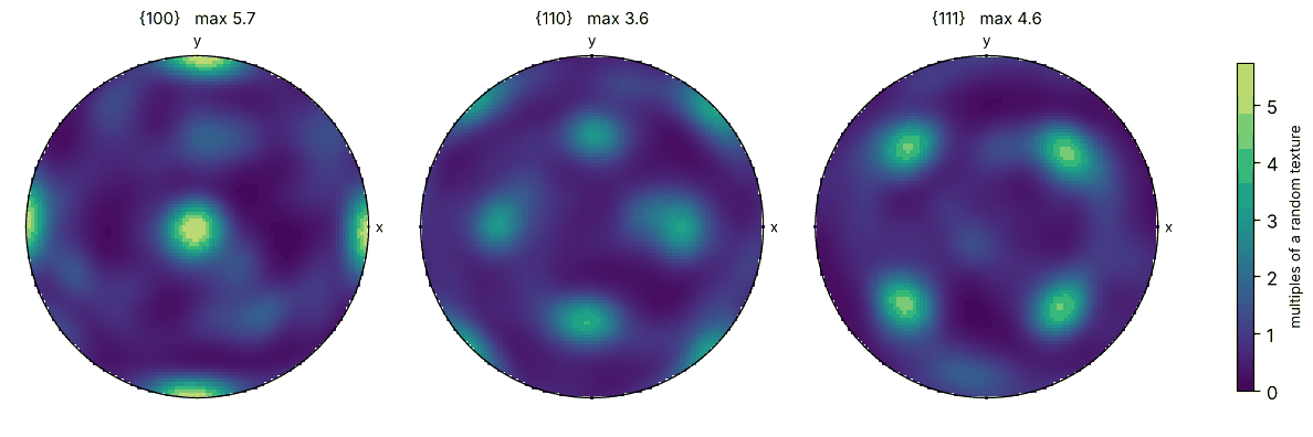
The {100} poles gather at the centre and on the two axes of the figure: two fifths of the area are within 15 degrees of the cube orientation. The boundaries tell the same:
pairs, lengths, angles = grains.boundaries()  # pairs of grains, lengths, disorientations
print(len(pairs), round(float(np.sum(lengths * angles) / lengths.sum()), 1))  # 130 38.4
Cubic crystals at random are 40.7 degrees apart on average (Mackenzie); here the
neighbours of the cube component are close to each other, and the mean is lower.
morphogen texture my_map.ctf -o texture/ prints these numbers and writes the tables of
the grains and of their boundaries with these figures.
3. The stiffness of its polycrystal¶
The grains of the map make a polycrystal of one cell through the thickness, each cell with the orientation of its grain — columns through the map, the third dimension being unknown. Its stiffness, with the elastic constants of nickel (GPa):
from morphogen.homogenization import Material, homogenize

crystals = grains.microstructure()
shape = (64, 48, 1)  # the points of the map
by_grain = {"grains": crystals.labels(shape).data, "orientations": crystals.orientations}
nickel = Material.cubic(246.5, 147.3, 124.7)
found = homogenize(crystals.voxelize(shape), {1: nickel}, properties=["stiffness"], **by_grain)
elastic = found["stiffness.periodic"]
print(round(elastic["bulk_modulus"], 2))  # 180.37 = (C11 + 2 C12) / 3, exactly
print(round(elastic["E1"], 1), round(elastic["E3"], 1))  # 188.5 197.8 GPa
The bulk modulus of a polycrystal of cubic crystals does not depend on their orientations. Its Young’s moduli do: with orientations at random the same grains give 227 GPa. A crystal of nickel is soft along its cube axes (136 GPa, for 304 along [111]), and the cube component brings these axes along those of the sample.
4. Into the plastic regime¶
The crystals slip on their twelve octahedral systems (the units are now megapascals). In finite strains the lattices turn with the slip. A tension to 2 % along the first axis, the other faces free, by the FFT solver of loading paths:
slipping = Material.from_config({
    "cubic": [246500, 147300, 124700],
    "crystal_plasticity": {"families": ["octahedral"], "tau0": 80.0, "Q": 20.0, "b": 10.0,
                           "K": 25.0, "n": 10.0},
})  # fmt: skip
path = {"times": [0, 20], "increments": 10, "strain": {"11": 0.02}}
results = homogenize(crystals.voxelize(shape), {1: slipping}, properties=[],
                     paths={"tension": path}, nonlinear={"kinematics": "finite"}, fields=True,
                     **by_grain)  # fmt: skip
pulled = results["tension.periodic"]
print(round(pulled.cauchy[-1, 0]))  # 251 MPa: the true stress at 2 %
euler, volumes = pulled.texture()  # the lattices of the crystals at the end, their volumes
start = crystals.orientations[by_grain["grains"].ravel()]
turned = texture.disorientation(euler, start)
print(round(turned.mean(), 2), round(turned.max(), 1))  # 0.71 2.6 degrees
At 2 % the lattices have turned by less than a degree on average, and not by the same
angle across a grain: the spread inside the grains grows with the strain. The fields of
a path written to files hold these orientations, and morphogen texture fields.vti -o texture/ draws their pole figures.
5. The lattices at a large strain¶
A texture forms over tens of percent. The simplest polycrystal is that of Taylor: every crystal undergoes the strain of the whole, here an extension of one half at constant volume, one material point per grain:
from morphogen.homogenization import simulate_point

stretch = np.linspace(1.0, 1.5, 11)
lateral = (stretch**-0.5 - 1.0).tolist()
zeros = [0.0] * len(stretch)
extension = {
    "times": np.linspace(0.0, 300.0, len(stretch)).tolist(),
    "increments": [4] * 10,
    "strain": {"11": (stretch - 1.0).tolist(), "22": lateral, "33": lateral,
               "23": zeros, "13": zeros, "12": zeros},
}  # fmt: skip
final = np.array([
    simulate_point(slipping, extension, orientation=e, kinematics="finite").orientation[-1]
    for e in grains.orientations
])  # fmt: skip
axis = (1.0, 0.0, 0.0)  # the direction of the extension
before = texture.inverse_pole_figure(grains.orientations, axis, weights=grains.areas)
after = texture.inverse_pole_figure(final, axis, weights=grains.areas)
print(round(before.at([1, 1, 1]), 1), round(after.at([1, 1, 1]), 1))  # 0.3 1.9
print(round(before.at([0, 1, 1]), 1), round(after.at([0, 1, 1]), 1))  # 0.8 0.3
fig = figures.inverse_pole_figure_figure(after, points=texture.inverse_poles(final, axis))
fig.savefig("texture_fibres.png")
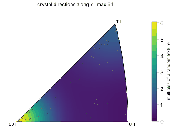
An inverse pole figure shows which direction of the crystals lies along a direction of the sample: here the axis of the extension, each point a grain. The axis leaves ⟨110⟩ and goes to ⟨111⟩ and to ⟨100⟩, the two fibres of the face-centred cubic metals in tension; the grains of the cube component were on the second one from the start, and stay there. In a compression the axis goes to ⟨110⟩. A crystal that slips on a single system turns as Schmid and Boas found, its tensile axis towards the slip direction: the tests of morphoGen check it to the elastic strains.
6. A polycrystal of space with the texture of the map¶
The map is a section, and its polycrystal is made of columns. Where the third dimension matters, a tessellation of space takes the texture of the map: each cell has the orientation of a grain of the map, drawn with the area of the grain, then turned by a few degrees so that 300 cells do not repeat 56 orientations.
textured = mg.models.Voronoi(
    n_cells=300,
    crystal_orientations=True,
    texture={"type": "measured", "file": "ebsd_map.ctf", "spread": 2.0},
)
polycrystal = textured.generate(mg.Domain.cube(10.0), seed=1)
cells = {"grains": polycrystal.labels(shape=24).data, "orientations": polycrystal.orientations}
found = homogenize(polycrystal.voxelize(shape=24), {1: nickel}, properties=["stiffness"], **cells)
solid = found["stiffness.periodic"]
print(round(solid["bulk_modulus"], 2))  # 180.37
print(round(solid["E1"], 1), round(solid["E3"], 1))  # 192.4 196.9 GPa
The polycrystal of space has the soft axes of the map (226 GPa with orientations at random), with grains of every shape instead of columns.
In a configuration file the two polycrystals are two models: {type: ebsd, file: my_map.ctf, window: random} takes a window of the map for each realization (the
template ebsd), and {type: voronoi, crystal_orientations: true, texture: {type: measured, file: my_map.ctf}} the tessellation; the file is taken from the folder of the
configuration.
Where to go next¶
The theory of each step — symmetries, disorientations, the kernel of the pole figures, the axes of the files, the rotation of the lattices: theory, §92.
The plasticity of the crystals, their twins and their cleavage: how a microstructure breaks.
The size of the windows of a map that represent it: how large is a representative volume?