Tutorial: exact geometry, from implicit functions to meshes¶
A realization of morphoGen is not an image: it is a description of the geometry (centres and radii, cells, layers…) from which every phase gets an implicit function, negative inside the phase, zero on its boundary, exact where the model puts its interfaces. Sections, surfaces and conforming meshes are cut from these functions at any resolution. This tutorial follows a composite of three phases — spheres, their interphase and the matrix — from its implicit functions to its surfaces (STL), its conforming mesh, whose quadratic elements bend along the interfaces, and three solvers on the same geometry: voxels, finite elements, and extended finite elements.
The snippets follow each other in one session and take about a minute and a half in
all, a third of it the mesher (MMG: the extra mesh).
1. A realization and its implicit functions¶
Non-overlapping spheres with a coating of constant thickness, in a periodic cube:
import numpy as np
import morphogen as mg
from morphogen.models import model_from_config

model = model_from_config(
    {
        "type": "coating",
        "model": {"type": "hardcore_spheres", "radius": 1.0, "volume_fraction": 0.2},
        "thickness": 0.3,
    }
)
micro = model.generate(mg.Domain.cube(5.0, periodic=True), seed=2)
print(micro.implicit_phases(), micro.summary())  # [0, 1, 2], 6 spheres
The exact volume fractions, to compare the discretizations with. The spheres do not overlap; their coatings do where two centres are closer than 2.6, and the interphase is the sum of the shells less the lenses that two coated spheres share (4.4 % of it here):
centres = micro.inner.spheres.centers
count = len(centres)
apart = centres[:, None, :] - centres[None, :, :]
apart -= 5.0 * np.round(apart / 5.0)  # through the faces of the periodic box
apart = np.linalg.norm(apart, axis=2)[np.triu_indices(count, 1)]
apart = apart[apart < 2.6]
lenses = np.sum(np.pi * (2.6 - apart) ** 2 * (apart + 5.2) / 12)
exact = {
    1: count * 4 / 3 * np.pi / 125,
    2: (count * 4 / 3 * np.pi * (1.3**3 - 1) - lenses) / 125,
}
print(exact)  # 0.2011 of spheres, 0.2300 of interphase
phase_level_set gives the implicit function of a phase at the centres of the voxels of
any grid: here the interphase (phase 2), the larger of the distance to the coated
spheres and of minus the distance to the spheres. Its sign is the phase of the voxel
image, at every point and at every resolution:
level = micro.phase_level_set(2, shape=48)  # negative inside the interphase
image = micro.voxelize(shape=48)  # phases 0 (matrix), 1 (spheres), 2 (interphase)
print(level.data.dtype, bool(((level.data < 0) == (image.data == 2)).all()))
mg.io.save_image(level, "interphase.vti")  # for ParaView: its zero level is the interface
Every model has such functions — the 39 models, their combinations, coatings, nested and
transformed structures: distances to unions of spheres and segments, differences of
power distances to the germs of cells, the rings of osteons, the leaves of a dead-leaves
model outside those that cover them (theory notes, §75). A structure of two
phases has one function, micro.level_set(...).
2. Sections at any resolution¶
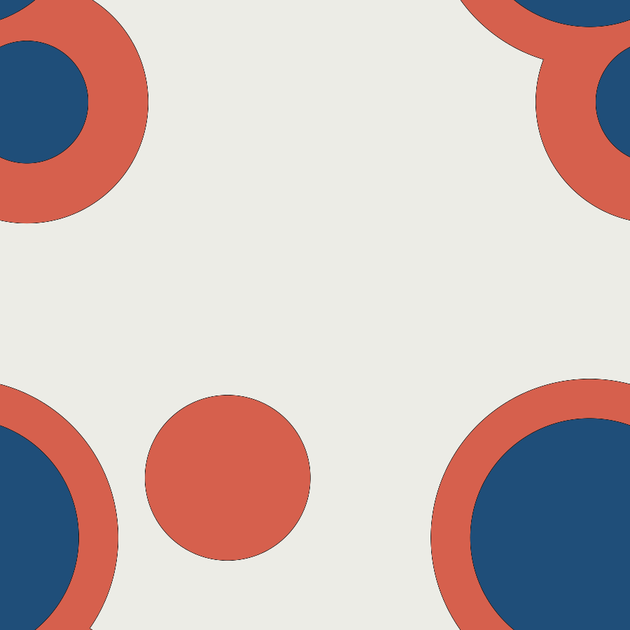
A section is computed in its plane, without the image of the volume: 900 × 900 pixels here, each with the fraction of the three phases that it holds (the anti-aliased boundaries of the figure), from the functions of the phases at the pixel centres.
from pathlib import Path

from morphogen.viz import encode_png, sections

cut = sections.section(micro, axis=2, fraction=0.5, resolution=900)
print(cut.shape, cut.sampling, sorted(cut.coverages))  # (900, 900) 'plane' [0, 1, 2]
Path("geometry_section.png").write_bytes(encode_png(sections.render(cut, contour=True)))
3. Surfaces¶
The surface of a phase is the zero level of its function (marching cubes on a grid), closed on the faces of the box: a watertight STL for a printer or a mesher. It converges to the volume of the spheres as the square of the spacing of the grid:
from morphogen.mesh.surface import surface_mesh

for n in (24, 48, 96):
    spheres = surface_mesh(micro.phase_level_set(1, shape=n), closed=True)
    print(n, len(spheres.faces), spheres.volume() / 125 / exact[1])  # 0.968, 0.992, 0.998
mg.io.save_mesh(spheres, "spheres.stl")
A configuration writes the same files with outputs: {surface: [stl], level_set: [vti]}
(one per phase for a structure of several phases), and the tab Export of the
graphical interface too.
4. A conforming mesh, and its quadratic elements¶
On a background grid (method="grid"), conforming_mesh cuts a mesh of the box by the
surfaces of the phases, one after the other, and remeshes it (MMG): tetrahedra whose
faces follow the two interfaces of each particle, with matching nodes on opposite faces
of the periodic box.
Nine pairs of coatings overlap here. They meet along grooves — sharp edges of the
interphase, which a function sampled on a grid would round over an element. The mesher
follows them: the coated spheres are cut in groups that do not overlap (the smooth
pieces of the structure, micro.implicit_pieces()), and the lines where two cuts meet
stay as edges of the mesh, flat.sharp.
flat = mg.mesh.conforming_mesh(micro, size=0.5, method="grid")  # size: the largest edge
print(flat.n_elements, flat.matching_faces(), float(flat.quality().min()))
print(flat.metadata["sharp_edges"], len(flat.sharp))  # 4 pieces, 270 sharp edges
fractions = flat.phase_fractions()
print(fractions[1] / exact[1], fractions[2] / exact[2])  # 0.963 and 0.993 of the volumes
These 4-node elements have flat faces: the mesh makes polyhedra of the spheres, inscribed
within the Hausdorff distance of the mesher (hausdorff, a twentieth of size), which
lose the volume between their chords and their surfaces. curved_mesh makes 10-node
elements of them and puts the nodes of the interfaces, corners and mid-edge nodes, on
the implicit surfaces — those of the sharp edges on the two surfaces that meet there:
the edges along the interfaces become arcs (isoparametric elements), the others stay
straight.
from morphogen.viz import figures

mesh = mg.mesh.curved_mesh(flat, micro)  # what conforming_mesh(..., order=2) returns
on = mesh.metadata["curved"]  # 22,800 of the 26,100 nodes of the interfaces lie on them
print(mesh.order, mesh.curved, on["nodes"], on["interface_nodes"], mesh.min_jacobian())
fractions = mesh.phase_fractions()
print(fractions[1] / exact[1], fractions[2] / exact[2])  # 1.0004 and 0.9990
mg.io.save_mesh(mesh, "coated.vtu")  # ParaView; also .mesh (Medit), .msh (Gmsh), .inp
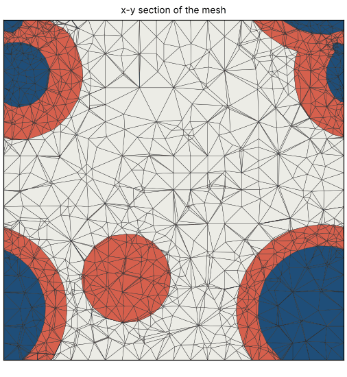
figures.mesh_figure(mesh).savefig("geometry_mesh.png", dpi=110)
The spheres and the interphase have their volumes back, within 0.1 %. With the grooves
rounded (sharp_edges=False: the box cut by the function of each phase, as for the
structures that do not give their pieces) the interphase would keep 0.9 % too much, in
the grooves, which no move of the nodes mends. The nodes that stay off their surfaces
are those that an element holds back, mostly in the gaps thinner than the grid of the
mesher between coatings that almost touch.
The 10-node elements are those of the finite element analyses: the 4-node ones are too
stiff, and lock when a phase flows plastically. A configuration takes them by default
for the meshes it analyses (mesh: {order: 1} for the 4-node ones, curved: false for
straight edges, sharp_edges: false for rounded grooves). phases="solid" leaves the pores of a porous medium out (their walls
are curved too), and the cells of a tessellation are meshed grain by grain with their
orientations; size sets the elements, background the grid on which the functions are
sampled for the mesher (half of size by default), which must resolve the thinnest gaps
and layers: here the interphase, of thickness 0.3.
By default (method: auto, without method="grid") the mesh is made without a grid,
from the functions of the phases at any point (an octree refined to the Hausdorff
distance, theory.md §94): the same grooves are followed, and the nodes of
the interfaces, those of the sharp edges on both surfaces, lie on them already with
4-node elements; the 10-node elements are curved by curved_mesh as above.
5. Three solvers on the same geometry¶
The finite elements of the conforming mesh, the FFT solver on voxels (whose interfaces are stairs) and the extended finite elements, which cut a regular grid by the level set instead of meshing it:
from morphogen.homogenization import LevelSetSample, Material, homogenize

materials = {
    0: Material(young=3.0, poisson=0.35),  # matrix
    1: Material(young=70.0, poisson=0.22),  # spheres
    2: Material(young=10.0, poisson=0.3),  # interphase
}


def bulk(sample, phases=materials, **options):
    out = homogenize(sample, phases, properties=["bulk_modulus"], **options)
    return out["bulk_modulus.periodic"].value


fe = {"4 nodes": bulk(flat, bcs=["periodic"]), "10 nodes": bulk(mesh, bcs=["periodic"])}
fft = {n: bulk(micro.voxelize(shape=n)) for n in (32, 64)}
print(fe, fft)  # 5.64 and 5.69; 5.82 and 5.75
The three approach the same value, about 5.69, each from its own side of the geometry. The voxels come down as their stairs get finer: 5.82 and 5.75 here, 5.72 at 128 and 5.70 at 192. The 10-node elements are there with elements of half the radius: 5.691, their phases at their volumes and their grooves sharp (5.725 with the grooves rounded, by the interphase that fills them). The 4-node elements give 5.640 on the same mesh, by two errors that hide each other in part — elements that are too stiff, spheres that have lost 4 % of their volume — and that do not always: under a plastic flow, or in the local fields, their stiffness is what is left. The bulk modulus of a cubic array of spheres has four digits with 10-node elements of the size of the radius (theory notes, §76, and §80 for the sharp edges).
The extended finite elements take the structures of two phases, here the spheres without their interphase, on a grid of 16 elements across, against voxels four times finer:
two = {0: materials[0], 1: materials[1]}
spheres_alone = micro.inner  # the structure that the coating covers
xfem = bulk(LevelSetSample.of(spheres_alone, 16), two)
voxels = bulk(spheres_alone.voxelize(shape=64), two)
print(xfem, voxels)  # 4.49 and 4.47
Which to choose: the FFT solver for speed and large volumes (periodic conditions, a GPU
if there is one); the conforming mesh, with its 10-node elements, for accurate
interfaces, the other boundary conditions (bcs=["kubc", "mixed", "subc"]) and cracks;
the extended finite elements for two-phase structures without a mesher. The
guide to the physics compares them problem by problem.
6. For other codes¶
mg.io.save_mesh(mesh, "coated.inp", materials=materials)  # Abaqus, CalculiX: sets, materials
mg.io.save_mesh(mesh, "coated.msh")  # Gmsh
mg.io.write_periodic_equations("coated_equations.inp", mesh)  # the periodic constraints
print(sorted(p.name for p in Path(".").glob("coated*")))
The template homogenization_interphase of the
gallery does all of this from a configuration (the
mesh, the level sets and surfaces of the phases, the finite elements), and the tool
Meshes and images in other formats of the tab Solvers & formats from the
interface.
Where next¶
The theory notes, §75: the implicit function of each kind of structure, the cuts of the mesher and their checks.
The gallery: the models, with the sections of their implicit functions.
A whole study and a rubber: the other tutorials.