Tutorial: a rubber, from its tests to its tearing¶
This tutorial follows a rubber through the finite strains of morphoGen: a hyperelastic law fitted to its tests, the law as a material at a point (with the softening of Mullins), a rubber filled with stiff particles stretched by half its length, and a cracked strip that tears at the stretch that Rivlin and Thomas predict. The first tutorial shows how to generate and characterize a morphology; this one starts where the strains stop being small.
The snippets follow each other in one session. The first three run in a second or two;
the filled rubber takes about forty seconds and the tearing about a minute (the first
run of a solver compiles its kernels, once). Strains and stresses are nominal in
finite strains: the strain E11 is the stretch minus one, the stress S11 the force
over the initial section; the results carry the true (logarithmic, Cauchy) measures
beside them (theory notes, §33).
1. The tests of a rubber¶
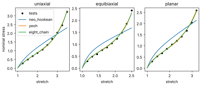
A rubber is tested in homogeneous states: uniaxial tension, equibiaxial tension (a sheet inflated or stretched in its plane) and planar tension (a wide strip, its width held: the pure shear test). Here the points of the three tests are those of a law we choose, with a scatter of 3 %; in a study they are your measures.
import numpy as np
from morphogen.homogenization import Hyperelasticity, Material, fit_hyperelasticity

chosen = Hyperelasticity("eight_chain", {"mu": 0.4, "lock": 2.5}).law(bulk=1000.0)
rng = np.random.default_rng(0)
tests = {}
for mode, top in (("uniaxial", 3.5), ("equibiaxial", 2.5), ("planar", 3.2)):
    stretch = np.linspace(1.0, top, 11)[1:]
    stress = chosen.nominal_stress(mode, stretch, incompressible=True)  # its closed form
    tests[mode] = (stretch, stress * (1.0 + 0.03 * rng.standard_normal(stretch.size)))
fit_hyperelasticity fits the parameters of a law to the tests together, by least
squares on the stresses of the incompressible solid:
fitted = {}
for model in ("neo_hookean", "mooney_rivlin", "yeoh", "eight_chain"):
    fitted[model] = fit_hyperelasticity(model, tests)
    law = fitted[model].law(bulk=1000.0)
    gaps = np.concatenate(
        [law.nominal_stress(m, lam, incompressible=True) / s - 1.0 for m, (lam, s) in tests.items()]
    )
    print(model, fitted[model].to_config(), f"{np.sqrt(np.mean(gaps**2)):.1%}")
The neo-Hookean and Mooney–Rivlin laws miss the points by about 30 %: they cannot stiffen
as the chains straighten. The polynomial of Yeoh (three coefficients of the first
invariant) and the eight chains of Arruda and Boyce follow them within the scatter, the
eight chains with the parameters we chose (mu 0.402 for 0.4, lock 2.51 for 2.5).
The other laws are fitted the same way — gent, van_der_waals, ogden (terms=3),
polynomial with the coefficients of start — and the fibres of soft tissues
(holzapfel), the foams (blatz_ko, hyperfoam) are given their parameters
(theory notes, §61).
from matplotlib.figure import Figure

fig = Figure(figsize=(7.5, 3.2), layout="constrained")
for ax, (mode, (stretch, stress)) in zip(fig.subplots(1, 3), tests.items(), strict=True):
    ax.plot(stretch, stress, "ko", ms=4, label="tests")
    fine = np.linspace(1.0, stretch[-1], 60)
    for model in ("neo_hookean", "yeoh", "eight_chain"):
        law = fitted[model].law(bulk=1000.0)
        ax.plot(fine, law.nominal_stress(mode, fine, incompressible=True), label=model)
    ax.set_title(mode)
    ax.set_xlabel("stretch")
fig.axes[0].set_ylabel("nominal stress")
fig.axes[0].legend()
fig.savefig("rubber_tests.png", dpi=110)
2. The law as a material¶
A material takes the law with a bulk modulus (the tests of an incompressible solid do not give it): its Young’s modulus and Poisson’s ratio at the natural state follow. We keep the polynomial of Yeoh for the rest of the study: its energy stays finite at any stretch, where the eight chains lock (near the tip of a crack the chains would).
from morphogen.homogenization import simulate_point

yeoh = {**fitted["yeoh"].to_config(), "bulk": 4.0}  # MPa
rubber = Material(hyperelasticity=yeoh)
print(rubber.young, rubber.poisson)  # 1.37 MPa and 0.44

cycle = {"times": [0, 1, 2, 3], "increments": [20, 10, 25], "strain": {"11": [0, 1.5, 0.1, 2.0]}}
soft = Material(hyperelasticity={**yeoh, "mullins": [1.5, 0.3, 0.1]})  # r, m, beta
point = simulate_point(soft, cycle, kinematics="finite")
first = point.stress[10, 0]  # at the stretch 1.75 of the first loading
again = np.interp(0.75, point.strain[30:, 0], point.stress[30:, 0])  # of the second
print(first, again, point.strain[20, 1])  # 0.63, then 0.24 MPa; the sides contract
simulate_point follows a loading path at a material point (homogeneous strain and
stress), the components that the path does not prescribe free of stress: a uniaxial
tension here, in which the sides contract by 31 % at a stretch of 2.5. mullins adds
the softening of filled rubbers (Ogden and Roxburgh): unloaded, the rubber is softer up
to the largest stretch it has seen, where it joins its first curve again. The same
material goes to every solver of loading paths: the voxels below, the finite elements of
a conforming mesh, the cracks of morphogen.fracture.
3. A filled rubber¶
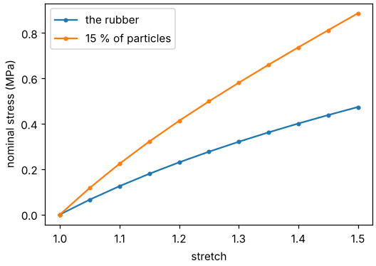
Stiff particles in the rubber — carbon black, silica — raise its stiffness more than their volume fraction: the rubber between them is stretched more than the composite. Non-overlapping spheres at 15 %, stretched by half their cell, the sides free:
import morphogen as mg
from morphogen.homogenization import homogenize

model = mg.models.HardcoreSpheres(radius=1.0, volume_fraction=0.15)
micro = model.generate(mg.Domain.cube(5.0, periodic=True), seed=3)
image = micro.voxelize(shape=16)
particles = Material(young=300.0, poisson=0.3)  # elastic: the energy of Hencky
pull = {"times": [0, 1], "increments": 10, "strain": {"11": [0, 0.5]}}
out = homogenize(
    image,
    {0: rubber, 1: particles},
    properties=[],
    paths={"pull": pull},
    nonlinear={"kinematics": "finite"},  # total Lagrangian, F-bar voxels
)
filled = out["pull.periodic"]
alone = simulate_point(rubber, pull, kinematics="finite")
fraction = float(np.mean(image.data == 1))
print(filled.stress[1, 0] / alone.stress[1, 0], 1 + 2.5 * fraction + 14.1 * fraction**2)
print(filled.cauchy[-1, 0], filled.log_strain[-1, 0])  # the true stress and strain
The composite carries 1.8 times the stress of the rubber alone on these 16³ voxels (3
per radius), and 1.62 times on 24³: finer voxels come to the estimate of Guth and Gold,
1 + 2.5 f + 14.1 f² ≈ 1.6 — resolve the particles before reading a curve. The
template homogenization_rubber of the gallery runs
such a composite through a cycle with the softening of Mullins; fields=True keeps the
fields of the voxels at the end of the path, and device="gpu" runs the solver on an
NVIDIA GPU.
fig = Figure(figsize=(4.8, 3.4), layout="constrained")
ax = fig.subplots()
ax.plot(1 + alone.strain[:, 0], alone.stress[:, 0], "o-", ms=3, label="the rubber")
ax.plot(1 + filled.strain[:, 0], filled.stress[:, 0], "o-", ms=3, label="15 % of particles")
ax.set_xlabel("stretch")
ax.set_ylabel("nominal stress (MPa)")
ax.legend()
fig.savefig("rubber_filled.png", dpi=110)
4. Tearing¶
How far can a cracked sheet be stretched? In the pure shear test — a strip of height
H with a long crack, stretched across it with its length held — the energy released
per unit area of crack is W(λ) H, with W the energy of the strip stretched to λ
far from the crack (Rivlin and Thomas 1953): the crack runs when it reaches the
toughness G_c. The energy W is the work of the material point along the same path:
held = {"11": [0, 0], "23": [0, 0], "13": [0, 0], "12": [0, 0]}
far = {
    "times": [0, 1],
    "increments": 200,
    "strain": {"22": [0, 1.0], **held},
    "stress": {"33": [0, 0]},
}
strip = simulate_point(rubber, far, kinematics="finite")
stretch = 1.0 + strip.strain[:, 1]
work = np.concatenate(
    [[0.0], np.cumsum(0.5 * (strip.stress[1:, 1] + strip.stress[:-1, 1]) * np.diff(stretch))]
)
The phase-field method breaks the cell without tracking the crack: a damage field
regularizes it over a length l, and each step of the path alternates the displacement
at fixed damage (the nonlinear FFT solver, its points degraded) and the damage of the
energy reached. On voxels of size h the toughness felt is G_c (1 + 3h / (8l)) (the
model AT1): we choose G_c so that the crack should run at a stretch of 1.6.
from morphogen.fracture import phase_field_fracture

nx, ny, critical = 36, 12, 1.6
h = 1.0 / ny  # the strip has the height H = 1
length = 2.0 * h
toughness = float(np.interp(critical, stretch, work)) / (1.0 + 3.0 * h / (8.0 * length))
sheet = mg.VoxelImage(np.zeros((nx, ny, 1), dtype=np.uint8), h, periodic=True)
crack = np.zeros((nx, ny, 1), dtype=bool)
crack[: nx // 2, ny // 2, 0] = True  # broken from the start: half the length
fracture = {"toughness": toughness, "length": length, "model": "AT1", "split": "volumetric"}
pull = {
    "times": [0, 1],
    "increments": 14,
    "strain": {"22": [0, 0.84], **held},
    "stress": {"33": [0, 0]},
}
torn = phase_field_fracture(
    sheet, {0: rubber}, fracture, pull, initial=crack, kinematics="finite", fields=True
)
stress = torn.stress[:, 1]
peak = int(np.argmax(stress))
broken = peak + int(np.flatnonzero(stress[peak:] < 0.1 * stress[peak])[0])
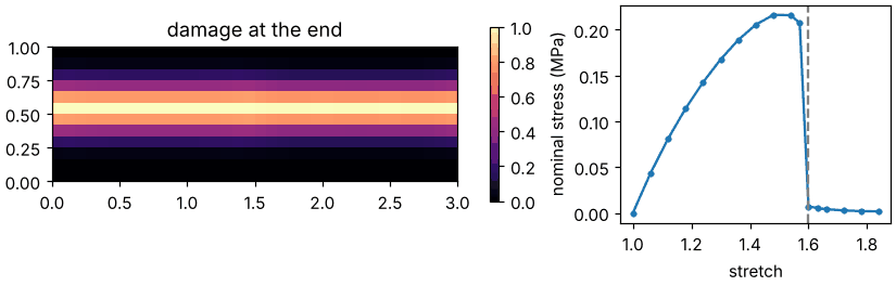
print(1 + torn.strain[peak, 1], 1 + torn.strain[broken, 1])  # 1.48 and 1.60, for 1.6
print(torn.crack_surface[-1], 1 + 3 * h / (8 * length))  # the area of the crack: 1.19
The crack starts at a stretch of 1.48 (the largest nominal stress) and has crossed the
cell at 1.60: the stretch of Rivlin and Thomas, within the size of the steps. Its
regularized area is that of the section of the strip times 1 + 3h / (8l). The split
volumetric lets the isochoric energy and the expansion break, so that a hydrostatic
compression does not; with elastic phases (no hyperelasticity: the energy of Hencky)
the split spectral of the small strains applies too. In small strains the same call
without kinematics runs the phase field of the guide to the physics;
the templates fracture_composite and fracture_rubber of the
gallery break a composite and a perforated sheet from a
configuration.
fig = Figure(figsize=(7.5, 2.4), layout="constrained")
left, right = fig.subplots(1, 2, width_ratios=(1.5, 1))
damage = torn.fields[1.0]["damage"][:, :, 0]  # of the voxels, at the end of the path
shown = left.imshow(
    damage.T, origin="lower", cmap="magma", vmin=0, vmax=1, extent=(0, nx * h, 0, 1)
)
left.set_title("damage at the end")
fig.colorbar(shown, ax=left, shrink=0.8)
right.plot(1 + torn.strain[:, 1], stress, "o-", ms=3)
right.axvline(critical, color="0.5", ls="--")  # the stretch of Rivlin and Thomas
right.set_xlabel("stretch")
right.set_ylabel("nominal stress (MPa)")
fig.savefig("rubber_torn.png", dpi=110)
Where next¶
The guide to the physics: every problem of the homogenization module, with the solver for each.
The theory notes: the strain energies and their checks (§61), the finite strains (§33), the phase field in small and finite strains (§64).
The tab Mechanics of the graphical interface: Material point and Loading path of a morphology take the same laws (search “strain energy” in its header); Fracture, Phase-field fracture of a morphology, the same phase field.