Tutorial: isogeometric analysis, from a patch to the shape of an auxetic sheet
In an isogeometric analysis the functions that describe the geometry — B-splines and
their rational form, NURBS — are also those of the unknowns. A circle is then a circle
whatever the number of elements, a refinement adds unknowns without touching the shape,
and the control points of the geometry are the natural variables of a shape
optimization: moving them moves the boundary smoothly, with no mesh to rebuild and
derivatives that are exact. This tutorial follows the package morphogen.iga from one
patch, checked against a closed form, to periodic cells (square, hexagonal, and cut
along no straight line at all), to the hole of largest bulk modulus, which reaches the
bound of Hashin and Shtrikman, and to a perforated sheet whose Poisson’s ratio the
optimizer drives to -0.8 at a given stiffness.
The snippets follow each other in one session and take about twenty seconds in all.
Everything here is in the plane (plane strain, or plane stress with plane="stress");
the same classes analyse solids (shapes.box, shapes.extruded).
1. A patch, and an exact solution to check it
A quarter of a thick-walled cylinder is one patch: quadratic and rational around the axis, where it is an exact arc, linear across the wall.
import math

import numpy as np

from morphogen import iga
from morphogen.homogenization import Material
from morphogen.iga import shapes

sheet = Material(young=1000.0, poisson=0.3, conductivity=2.0)
ring = shapes.annulus(1.0, 2.0)  # a quarter of the ring between the radii 1 and 2
inner = ring.side(1, 0).sample(64)  # points of its inner side
print(ring.degrees, ring.shape)  # (2, 1) (3, 2): 6 control points
print(np.abs(np.linalg.norm(inner, axis=1) - 1.0).max())  # 1e-16
The points of its inner side are at the radius 1 to round-off: the geometry is exact
with six control points. Under an internal pressure the radial displacement is that of
Lamé; the refinements below keep the geometry and raise the degree across the wall to 2
(elevate), then cut each element in 2, 4 and 8:
def lame(points, inner=1.0, outer=2.0, pressure=1.0):
    """The displacement of Lamé's cylinder in plane strain."""
    r = np.linalg.norm(points, axis=1)
    factor = (1 + sheet.poisson) * pressure * inner**2 / (sheet.young * (outer**2 - inner**2))
    radial = factor * ((1 - 2 * sheet.poisson) * r + outer**2 / r)
    return radial[:, None] * points / r[:, None]


errors = {}
for subdivisions in (2, 4, 8):
    model = iga.Multipatch(ring.refined(subdivisions, elevate=(0, 1)))
    analysis = iga.Analysis(model, {0: sheet})  # plane strain
    x = model.nodes
    fixed = np.concatenate(
        [
            analysis.dofs(np.flatnonzero(np.abs(x[:, 1]) < 1e-12), [1]),  # u_y = 0 on y = 0
            analysis.dofs(np.flatnonzero(np.abs(x[:, 0]) < 1e-12), [0]),  # u_x = 0 on x = 0
        ]
    )
    # the pressure on the inner side: patch 0, direction 1 (across the wall), its start
    forces = analysis.side_load(0, 1, 0, lambda points, normals: -1.0 * normals)
    u = analysis.solve(forces, fixed)
    errors[subdivisions] = analysis.error(u, lame)["l2"]
print(errors)  # 1.7e-3, 2.0e-4, 2.4e-5: divided by 8 at each halving
The error of the displacement is divided by eight each time the elements are halved:
the third order of quadratic functions, with 32, 72 and 200 unknowns. With cubic
functions (elevate=(1, 2)) it is the fourth order, and less than 2e-6 with 242
unknowns.
2. Periodic cells: a box, a rhombus
A cell with a hole is four patches around it, each from a side of the cell to the arc that faces it. Opposite sides have matching control points, and equal unknowns there make the fields periodic exactly. The effective stiffness of a sheet with a square array of circular holes, in plane strain:
cell = shapes.cell_with_hole((1.0, 1.0), 0.3)
solid = iga.homogenize(cell.refined(8, (1, 2)), {0: sheet})
print(solid.fraction, 1 - math.pi * 0.3**2)  # 0.71725666 both: the hole is a circle
print(solid.tensor.round(1))  # C11 = C22 = 618.8, C12 = 187.1, C66 = 132.6
print(solid.constants())  # Young's moduli, Poisson's ratios, shear and bulk moduli of the plane
For conduction there is a closed form to compare with: the series of Perrins, McKenzie
and McPhedran (1979) for arrays of cylinders, here non-conducting ones. The hexagonal
array has a rhombus as its cell — cell_with_hole takes the two vectors of an oblique
lattice in place of the lengths of a box, and the assembly carries them as its
lattice:
def perrins(holes, array):
    """The conductivity of a sheet with an array of circular holes, over that of the sheet."""
    f = holes
    if array == "square":
        return 1 - 2 * f / (1 + f - 0.305827 * f**4 / (1 - 1.402958 * f**8) - 0.013362 * f**8)
    return 1 - 2 * f / (1 + f - 0.075422 * f**6 / (1 - 1.060283 * f**12) - 0.000076 * f**12)


square = iga.homogenize(cell.refined(8, (1, 2)), {0: sheet}, physics="conduction")
rhombus = shapes.cell_with_hole([[1.0, 0.0], [0.5, math.sqrt(0.75)]], 0.4)
hexagonal = iga.homogenize(rhombus.refined(8, (1, 2)), {0: sheet}, physics="conduction")
holes = 1 - hexagonal.fraction
print(square.tensor[0, 0] / 2, perrins(math.pi * 0.09, "square"))  # 0.558486, 0.558485
print(np.diag(hexagonal.tensor) / 2, perrins(holes, "hexagonal"))  # 0.26415 twice, 0.264145
print(1 - 2 * holes / (1 + holes))  # 0.26549: the estimate of Maxwell, 0.5 % above
The two conductivities of the hexagonal array are equal, as its symmetry wants, and
equal to the series within 0.002 %. Its elastic stiffness is isotropic too: C_66 = (C_11 - C_12) / 2 within 0.06 % on this grid, and closer with each refinement.
A cell need not even be a parallelogram: any set of patches that tiles the plane by the
periods of its lattice will do, the control points of its boundary that are a period
apart being one. Section 4 uses that for a pattern whose natural pieces are cut by no
straight line.
3. The hole of largest bulk modulus
A design is a coarse assembly whose control points the variables move; its analysis is
a refinement of it, whose control points follow linearly. Here the hole of a square
cell takes 40 % of its area, and three variables scale the distances of its control
points to the centre, with the symmetries of the square ("d4"). The derivatives of the
effective stiffness with respect to the variables are analytical — one integral of the
energy-momentum tensor of Eshelby per pair of loadings, no further solution.
from morphogen.iga import optimization as opt

porosity = 0.4
cell = shapes.cell_with_hole((1.0, 1.0), math.sqrt(porosity / math.pi), elements=4)
design = opt.ShapeDesign(cell, subdivisions=4, elevate=(1, 2))
hole = np.unique(np.concatenate([cell.side_nodes(k, 1, 1) for k in range(4)]))
design.radial(hole, (0.5, 0.5), -0.3, 0.3, symmetry="d4")
matrix = iga.elastic_matrix(sheet, 2, "strain")
bulk, shear = 0.5 * (matrix[0, 0] + matrix[0, 1]), matrix[2, 2]
bound = bulk * shear * (1 - porosity) / (shear + porosity * bulk)  # Hashin and Shtrikman

stiffest = opt.optimize_cell(
    design,
    {0: sheet},
    lambda c, f: -iga.plane_constants(c)["bulk_modulus"] / bulk,  # to minimize
    [lambda c, f: f / (1 - porosity) - 1.0],  # the material kept: f <= 0.6
    tolerance=1e-10,
)
circle = iga.plane_constants(opt.cell_response(design, np.zeros(3), {0: sheet}).tensor)
best = iga.plane_constants(stiffest.tensor)
print(design.n, design.fine.n_nodes, stiffest.iterations)  # 3 variables, 588 control points, 7
print(circle["bulk_modulus"] / bound, best["bulk_modulus"] / bound)  # 0.9861, 0.99995
The circle is 1.4 % below the upper bound of Hashin and Shtrikman for the bulk modulus of a porous sheet; in seven iterations the optimizer finds the rounded square of Vigdergauz (1994), which attains it — within 0.005 % here.
import matplotlib

matplotlib.use("Agg")
import matplotlib.pyplot as plt

fig, axes = plt.subplots(1, 2, figsize=(7.0, 3.6))
for ax, model, title in (
    (axes[0], cell, f"circle: {circle['bulk_modulus'] / bound:.3f} of the bound"),
    (axes[1], stiffest.design, f"optimized: {best['bulk_modulus'] / bound:.3f} of the bound"),
):
    for polygon in model.polygons(24):
        ax.fill(polygon[:, 0], polygon[:, 1], color="#c9d6e3", lw=0.4)
    for line in model.outline(24):
        ax.plot(line[:, 0], line[:, 1], color="#34495e", lw=0.6)
    ax.plot(model.nodes[hole, 0], model.nodes[hole, 1], "o", color="#c0392b", ms=3)
    ax.set(aspect="equal", title=title)
    ax.axis("off")
fig.tight_layout()
fig.savefig("iga_hole.png", dpi=110)
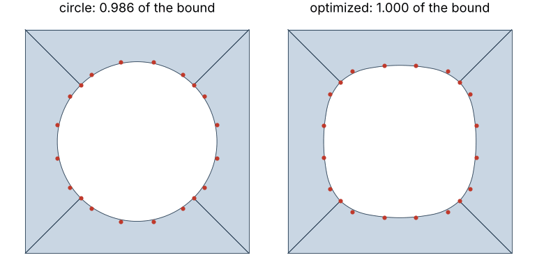
The patches of the design with the control points of the hole: on the right they have moved to the hole of largest bulk modulus.
4. An auxetic sheet
Cut elongated holes at the nodes of a square lattice, in turn along its two axes. The squares of sheet left between four holes hold together by the ligaments between the tip of a hole and the flank of the next; when the ligaments are thin the squares turn rather than stretch, and the sheet widens when it is pulled — the rotating squares (Grima & Evans 2000; Bertoldi et al. 2010; Taylor et al. 2014).
The natural pieces of this pattern are the squares, which no straight line separates.
alternating_holes returns two of them, whole, as the cell of the oblique lattice
(1, 1), (1, -1): sixteen patches, the holes exact ellipses. In plane stress, for holes
0.06 wide and longer and longer:
ligaments, ratios, moduli = [], [], []
for a in (0.3, 0.4, 0.5, 0.6, 0.7, 0.8, 0.85, 0.9):
    grains = shapes.alternating_holes(1.0, (a, 0.03))  # the half-axes along and across
    out = iga.homogenize(grains.refined(4, (1, 2)), {0: sheet}, plane="stress")
    constants = out.constants()
    ligaments.append(1.0 - a - 0.03)
    ratios.append(constants["poisson_12"])
    moduli.append(constants["young_1"])
print(
    grains.lattice, len(grains.patches), out.tensor[0, 2] / out.tensor[0, 0]
)  # 16 patches, ~1e-12
print(np.round(ratios, 3))  # 0.187 0.031 -0.211 -0.487 -0.722 -0.883 -0.937 -0.975
Poisson’s ratio changes sign when the ligaments are a little more than half the
spacing and tends to -1 as they thin, while Young’s modulus falls from 731 to 3.5 (1000
for the plain sheet). The stiffness keeps the
symmetries of the square (C_16 = 0, C_11 = C_22), and with circular holes it is that
of the box of section 2 to seven digits.
The most auxetic sheet of a given stiffness. Two variables are enough: the half-axes
of the holes, of all the holes together. A variable moves control points of the design
along directions; with the symmetry of the pattern — its two mirrors through a hole
and the quarter-turn about the centre of a square — it moves their images as well, and
the control points of the boundary of the cell that are a period apart. The patches 0
and 1 are those of the hole at the origin: their first rows of control points are its
arc, and the others follow the middles of the ligaments.
a, b = 0.6, 0.1
grains = shapes.alternating_holes(1.0, (a, b))
design = opt.ShapeDesign(grains, subdivisions=4, elevate=(1, 2))
flank, tip = grains.ids[0], grains.ids[1]  # the patches of the hole at the origin
arc = np.unique(np.concatenate([flank[:, 0], tip[:, 0]]))
symmetry = [opt.mirror(0), opt.mirror(1), opt.rotation(90.0, (0.5, 0.5))]
x = grains.nodes
# the hole stretched along its axis: the middle of the ligament at its tip moves by half
along = [*(x[arc] * [1 / a, 0.0]), [0.5, 0.0], [0.5, 0.0]]
design.variable([*arc, *tip[1:, 1]], along, -0.2, 0.25, "a", symmetry=symmetry)
# and across: the middle of the ligament at its flank
across = [*(x[arc] * [0.0, 1 / b]), [0.0, 0.5], [0.0, 0.5]]
design.variable([*arc, *flank[:2, 1]], across, 0.03 - b, 0.1, "b", symmetry=symmetry)
print(design.n, [len(nodes) for nodes, _ in design.moves])  # 2 variables of 53 control points


def ratio(c, f):
    return iga.plane_constants(c)["poisson_12"]


auxetic = opt.optimize_cell(
    design,
    {0: sheet},
    ratio,
    [lambda c, f: 1.0 - iga.plane_constants(c)["young_1"] / 50.0],  # E_1 >= 50
    linear=([[1.0, 1.0]], [1.0 - a - b - 0.05]),  # ligaments of 0.05 at least
    plane="stress",
    tolerance=1e-10,
)
found = iga.plane_constants(auxetic.tensor)
print(auxetic.iterations, a + auxetic.x[0], b + auxetic.x[1])  # 8 iterations: 0.751 and 0.03
print(found["poisson_12"], found["young_1"])  # -0.814 and 50.0
From the holes 0.6 by 0.1 (a ratio of -0.53, a modulus of 157) the optimizer goes in
eight iterations to slits of the least width allowed (the lower bound of b), long
enough for the modulus to come down to its bound: 0.751 by 0.03, and a ratio of -0.814.
The bounds of the variables are those of the process that cuts the sheet; linear
adds linear constraints on the variables, here the width of the ligaments (the control
points being linear in the variables, so are the sizes of the geometry). A finer
analysis of the design confirms the values:
check = iga.homogenize(auxetic.design.refined(8, (1, 2)), {0: sheet}, plane="stress")
print(check.analysis.n_dofs, check.constants()["poisson_12"], check.constants()["young_1"])
# 3482 unknowns: -0.816 and 49.5
fig, axes = plt.subplots(1, 3, figsize=(10.5, 3.6))
for ax, model, title in (
    (axes[0], grains, "holes 0.6 x 0.1: ratio -0.53"),
    (axes[1], auxetic.design, f"optimized: ratio {found['poisson_12']:.2f}"),
):
    tiles = shapes.repeated(model, (2, 2))  # the cell and three neighbours
    for polygon in tiles.polygons(16):
        ax.fill(polygon[:, 0], polygon[:, 1], color="#c9d6e3", lw=0.4)
    for polygon in model.polygons(16):
        ax.fill(polygon[:, 0], polygon[:, 1], color="#7f9fbf", lw=0.4)
    ax.set(aspect="equal", title=title, xlim=(0.4, 3.6), ylim=(-0.6, 1.6))
    ax.axis("off")
axes[2].plot(ligaments, ratios, "o-", color="#34495e", label="ellipses 0.06 wide")
ligament = 1 - a - b - auxetic.x.sum()
axes[2].plot(ligament, found["poisson_12"], "s", color="#c0392b", label="optimized")
axes[2].axhline(0.0, color="0.6", lw=0.6)
axes[2].set(xlabel="ligament / spacing", ylabel="Poisson's ratio")
axes[2].legend(frameon=False)
fig.tight_layout()
fig.savefig("iga_auxetic.png", dpi=110)
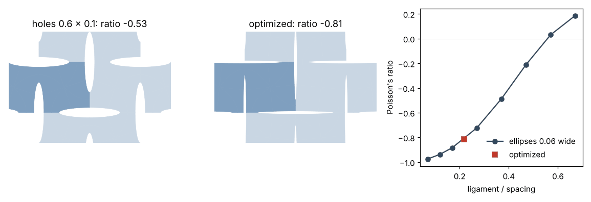
The cell (darker: two squares, sixteen patches) among its neighbours, before and after; Poisson’s ratio against the width of the ligaments.
The same sheet for the other solvers. An assembly of patches gives its image on a grid, with the copies of its patches by the periods of its lattice: over a box that is a period of the medium — here the square of four holes — the image is periodic, and goes to the voxel solvers, to the nonlinear behaviours and to the exports like any other microstructure. The FFT solver on the optimized sheet, against the isogeometric analysis in plane strain:
from morphogen.homogenization import homogenize

voxels = auxetic.design.voxelize((256, 256), lower=(0.0, 0.0), upper=(2.0, 2.0))
by_fft = homogenize(voxels, {0: sheet, 1: Material(void=True)}, properties=["stiffness"])
by_fft = by_fft["stiffness.periodic"]["tensor"][np.ix_([0, 1, 5], [0, 1, 5])]
by_iga = iga.homogenize(auxetic.design.refined(8, (1, 2)), {0: sheet}).tensor
print(by_fft[[0, 0, 2], [0, 1, 2]].round(1))  # C11, C12, C66 of the image: 160.7, -128.6, 85.0
print(by_iga[[0, 0, 2], [0, 1, 2]].round(1))  # and of the patches: 157.5, -127.5, 85.4
Two methods that share nothing agree within 2 % — the image has eight pixels across a
slit —, and both give a negative C_12.
What decides the ratio. Freeing the shape of the holes further — the fullness of their tips and of their flanks, two more variables linked in the same way — gains nothing here: at a given stiffness the ratio of this pattern is that of its ligaments, whatever the outline of the holes away from them (-0.8142 against -0.8141). An honest optimizer says so; it is the width of the ligaments and of the slits, the limits of the process, that set what the sheet can do.
Inverse design. The same two variables find the holes that give a sheet prescribed constants. With the distance to a goal as the objective — say the modulus and the ratio of the holes 0.7 by 0.07 —, the optimizer finds these holes again from 0.6 by 0.1, to six digits:
goal = iga.plane_constants(
    opt.cell_response(design, np.array([0.1, -0.03]), {0: sheet}, plane="stress").tensor
)


def distance(c, f):
    k = iga.plane_constants(c)
    return (k["young_1"] / goal["young_1"] - 1) ** 2 + (k["poisson_12"] - goal["poisson_12"]) ** 2


inverse = opt.optimize_cell(design, {0: sheet}, distance, plane="stress", tolerance=1e-14)
print(goal["young_1"], goal["poisson_12"])  # 68.0 and -0.755
print(inverse.x, inverse.objective)  # [0.1, -0.03] and 2e-17
Where to go next
The notes of theory give the formulas: isogeometric analysis (the bases, the patches, the refinements, the periodic cells) and its shape optimization (the derivatives, the optimizers, the benchmarks with closed forms).
optimize_structureminimizes the compliance of a structure under loads: the hole of a plate under biaxial tension becomes the ellipse of the infinite plate.method="mma"uses the method of moving asymptotes in place of sequential quadratic programming;physics="conduction"optimizes conductivities with the same calls.Your own patterns: build the patches with
shapes.ruledbetween two curves, assemble them withiga.Multipatch(patches, lattice=...), and link the variables by the symmetries of the pattern.