Tutorial: a whole study¶
This tutorial follows one microstructure from its generation to a behaviour learned from its responses: SiC particles in an aluminium alloy, the particles a Boolean model of spheres. It generates the morphology (from the command line, from Python and in the graphical interface), characterizes it (volume fraction, covariance, percolation threshold), computes its apparent elastic properties by the FFT solver and the size of its representative volume element, follows a loading path with a von Mises matrix, exports it for other codes (MFront, Abaqus, AMITEX_FFTP) and learns its behaviour.
The Python snippets follow each other in one session (python, IPython or a notebook)
and each runs in seconds, at sizes chosen for that; the first run of each solver compiles
its kernels (up to a minute or two, once: the compiled code is cached). The figures are
those that the snippets save. The gallery shows the other models, the
user guide each step, and the theory notes the formulas behind the
results; the other tutorials measure the size of the representative
volume, follow a rubber to its tearing and the exact geometry of a composite to its
meshes, and tour the graphical interface.
1. Install¶
morphoGen needs Python 3.12 or newer; every dependency comes as a binary wheel. In a virtual environment (see Installation for uv, conda, the GPU and MFront):
git clone https://github.com/jdirr/morphoGen.git
cd morphoGen
python -m venv .venv
.venv\Scripts\activate          # Windows; source .venv/bin/activate on macOS and Linux
python -m pip install -e ".[all]"
morphogen info                  # versions, threads, the mesher, the GPU and MFront found
2. Generate a morphology¶
From the command line¶
A run is described by a configuration file: the model, the domain, the voxels, the
outputs and the measures. The templates are examples to start from (morphogen template
lists them, the gallery shows them):
morphogen models                                   # the models
morphogen models boolean_spheres                   # the parameters of one
morphogen template boolean_spheres -o spheres.yaml
Edit spheres.yaml down to the study of this tutorial: spheres of radius 1 filling 20 %
of a periodic cube of edge 10, voxelized at 64³:
model:
  type: boolean_spheres
  radius: 1.0
  volume_fraction: 0.2
domain:
  size: 10.0
  periodic: true
seed: 1
voxels:
  shape: 64
outputs:
  directory: out/spheres
  name: spheres
  geometry: [json]               # the explicit geometry: centres and radii
  image: [vti]                   # the voxels, for ParaView and the FFT solvers
analysis: [volume_fraction, specific_surface, connectivity]
morphogen run spheres.yaml                          # out/spheres: files, results.csv, run.json
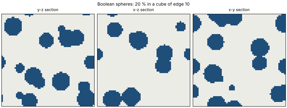
morphogen view out/spheres/spheres_0000.vti         # its three middle sections (a PNG)
results.csv holds the measures of each realization, run.json the configuration and
the theory of the model (here its volume fraction, specific surface and integral range).
From Python¶
The same realization: the realizations of a run take the seeds derived from its seed,
derive_seed(seed, i) for the realization i.
import morphogen as mg
from morphogen.seeding import derive_seed

model = mg.models.BooleanSpheres(radius=1.0, volume_fraction=0.2)
domain = mg.Domain.cube(10.0, periodic=True)
micro = model.generate(domain, seed=derive_seed(1, 0))  # the realization 0 of seed 1
image = micro.voxelize(shape=64)  # 64³ voxels of phases 0 (matrix) and 1 (spheres)
print(micro.summary())  # {'n_spheres': 58}
mg.io.save_image(image, "spheres.vti")
micro is the explicit description of the realization (centres and radii), which
mg.io.save_microstructure(micro, "spheres.json") keeps and regenerates exactly; it can
be voxelized at any resolution and meshed conformingly (mg.mesh.conforming_mesh, with
the extra mesh: see the tutorial on exact geometry). Its three
middle sections, as a figure (matplotlib, the extra plot):
from morphogen.viz import figures

fig = figures.slices_figure(image, title="Boolean spheres: 20 % in a cube of edge 10")
fig.savefig("study_sections.png", dpi=110)
In the graphical interface¶
morphogen gui opens the interface in the web browser. In Create, tab Generate,
choose boolean_spheres in the menu of the models on the left (family Random sets and
particles; the filter above it finds a model by a word of its name or summary): its
form opens filled with its template; set the radius to 1, the volume fraction to 0.2,
the edge of the domain to 10 and the seed to 1, then Generate (or Ctrl + Enter).
The page shows the sections of the realization, its summary and its measures against
the theory of the model, and keeps the morphology in the workspace, the strip below
the menus, from which every other tab takes it: Characterize (Statistics: measures,
correlation functions, percolation threshold, RVE size), Simulate (Linear
homogenization, Mechanics, Fracture, Physics…) and Export & compare (Export,
Solvers & formats). Each of these tabs lists its tools on its left; the search of the
header (/) finds a tool, a model or an option of a form by a word (“percolation”,
“gyroid”, “ogden”) and opens it; ? shows the map of the interface. View in 3D,
in the menu of its chip, turns the morphology in the page. The interface runs the same
functions as the snippets below.
3. Characterize it¶
The measures of the image against the closed forms of the model (theory notes, §1):
from morphogen import analysis

theory = model.theory(domain)
print(analysis.volume_fraction(image), theory["volume_fraction"])  # 0.219 against 0.2
print(analysis.specific_surface(image), theory["specific_surface"])
lags, values = analysis.covariance(image).mean()  # along x, y and z, then their mean
print(values[:4], model.covariance(lags[:4]))  # C(h) = P(x and x + h in the spheres)
print(theory["integral_range"])  # 3.88: the RVE grows with it
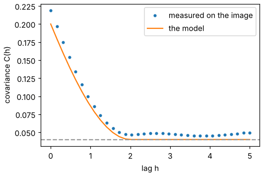
The volume fraction of one realization in a small box differs from that of the model by a few hundredths: section 4 measures how this scatter falls with the volume. The covariance of the image against that of the model, which falls from the volume fraction to its square over the diameter of the spheres:
from matplotlib.figure import Figure

fig = Figure(figsize=(4.8, 3.2), layout="constrained")
ax = fig.subplots()
ax.plot(lags, values, "o", ms=3, label="measured on the image")
ax.plot(lags, model.covariance(lags), label="the model")
ax.axhline(theory["volume_fraction"] ** 2, color="0.6", ls="--")  # its asymptote
ax.set_xlabel("lag h")
ax.set_ylabel("covariance C(h)")
ax.legend()
fig.savefig("study_covariance.png", dpi=110)
The spheres percolate (a cluster of them joins opposite faces) above a critical volume
fraction. percolation_threshold bisects the fraction at which half of the realizations
percolate, the realizations drawn from a configuration at each fraction:
from morphogen.analysis.percolation import family_from_config, percolation_threshold

config = {
    "model": {"type": "boolean_spheres", "radius": 1.0, "volume_fraction": 0.2},
    "domain": {"size": 16.0, "periodic": True},
    "voxels": {"shape": 64},
}
family = family_from_config(config)  # a realization at any volume fraction
found = percolation_threshold(family, 0.15, 0.45, seed=0)
print(found.threshold, found.bracket)  # about 0.27
The threshold of overlapping spheres in the continuum is 0.2895; the voxels lower it
(spheres closer than about a voxel touch on the image), to 0.27 at 4 voxels per radius
(theory notes, §55). The command line does the same with the domain and voxels of a
configuration, and percolation_scaling (--sizes) extrapolates the thresholds of
growing boxes to the infinite medium:
morphogen percolation spheres.yaml --lower 0.15 --upper 0.45
4. Apparent elastic properties and the RVE¶
The FFT solver homogenizes voxel images under periodic conditions (on an NVIDIA GPU with
device="gpu" and the extra gpu):
from morphogen.homogenization import Material, bounds, homogenize

alloy = Material(young=70e3, poisson=0.33)  # the aluminium alloy (MPa)
sic = Material(young=400e3, poisson=0.2)  # the SiC particles
materials = {0: alloy, 1: sic}
results = homogenize(image, materials, properties=["bulk_modulus", "shear_modulus"])
mu = results["shear_modulus.periodic"].value
hs = bounds(analysis.phase_fractions(image), materials)["shear_modulus"]
print(mu, hs["hs_lower"], hs["hs_upper"])  # 38.1 GPa, within 36.7 and 45.9
properties=["stiffness"] gives the whole stiffness tensor, loadings mixed macroscopic
strains and stresses, and mg.mesh.conforming_mesh with bcs=["kubc", "mixed", "periodic", "subc"] the finite elements on conforming meshes.
How large must a volume be for its apparent modulus to stand for the material? The
statistical method of Kanit et al. (2003) computes the modulus of realizations of
several volumes V, fits the variance as D²(V) = K V^-γ and gives the volume whose
mean over n realizations reaches a relative error ε (theory notes, §9):
import numpy as np
from morphogen import rve

volumes, moduli = [], []
for size in (4.0, 6.0, 8.0):  # edges of the volumes
    box = mg.Domain.cube(size, periodic=True)
    for r in range(16):  # realizations of each volume
        sample = model.generate(box, seed=derive_seed(2, int(size), r))
        voxels = sample.voxelize(voxel_size=0.25)  # the same voxel size at every volume
        out = homogenize(voxels, materials, properties=["shear_modulus"])
        volumes.append(size**3)
        moduli.append(out["shear_modulus.periodic"].value)
stats = rve.ensemble_statistics(volumes, moduli)  # mean and variance of each volume
law = rve.fit_statistics(stats, gamma=1.0)  # K, with gamma = 1 for this model
for row in rve.rve_table(law, np.mean(moduli)):
    print(row)  # the volume and edge for 1 and 5 %, with 1 and 10 realizations
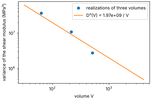
The variance of the apparent modulus against the volume, with the law fitted to it: a line of slope -1 on logarithmic axes, as for every medium whose correlations have a finite range (theory notes, §9), from which the table reads the volume of a precision. The points scatter about it: a variance estimated from 16 realizations is known within a third.
fig = Figure(figsize=(4.8, 3.2), layout="constrained")
ax = fig.subplots()
ax.loglog(stats.volume, stats.variance, "o", label="realizations of three volumes")
grid = np.geomspace(stats.volume.min() / 2, stats.volume.max() * 8, 30)
ax.loglog(grid, law.variance(grid), label=f"D²(V) = {law.K:.3g} / V")
ax.set_xlabel("volume V")
ax.set_ylabel("variance of the shear modulus (MPa²)")
ax.legend()
fig.savefig("study_rve.png", dpi=110)
A configuration with an rve section runs such a study, in parallel (-j) or on a
cluster (morphogen submit), and writes its report (rve_report.md, with confidence
intervals and figures): the tutorial how large is a representative
volume? runs one, and the templates rve_poisson_fibers and
rve_crystal_plasticity_fft of the gallery are others.
5. A nonlinear loading path¶
Now the matrix yields: von Mises elasto-plasticity with a Voce isotropic hardening. A loading path prescribes components of the macroscopic strain or stress in time and leaves the others free of stress: here a tension to 1 % in 10 increments, the lateral faces free:
from morphogen.homogenization import LoadingPath, simulate_point

alloy = Material(
    young=70e3, poisson=0.33, plasticity={"yield": 100, "isotropic": [{"Q": 80, "b": 20}]}
)  # von Mises, Voce
path = LoadingPath.parse("t=0,1 n=10 E11=0,0.01")
coarse = micro.voxelize(shape=16)  # 16³ voxels: seconds
out = homogenize(coarse, {0: alloy, 1: sic}, properties=[], paths={"tension": path})
curve = out["tension.periodic"]  # times, strains, stresses, plastic strain of the phases
print(curve.stress[-1, 0], simulate_point(alloy, path).stress[-1, 0])  # composite, matrix
matrix = simulate_point(alloy, path)
fig = Figure(figsize=(4.8, 3.2), layout="constrained")
ax = fig.subplots()
ax.plot(curve.strain[:, 0], curve.stress[:, 0], "o-", ms=3, label="composite (16³ voxels)")
ax.plot(matrix.strain[:, 0], matrix.stress[:, 0], "o-", ms=3, label="matrix alone")
ax.set_xlabel("strain 11")
ax.set_ylabel("stress 11 (MPa)")
ax.legend()
fig.savefig("study_tension.png", dpi=110)
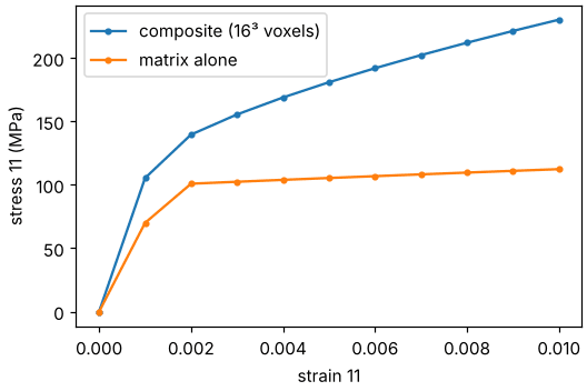
The particles carry a growing share of the load as the matrix yields: on these 16³
voxels (1.6 per radius) the composite reaches about twice the stress of the matrix alone
(simulate_point: the material point under the same path), but finer voxels lower the
ratio (1.7 on 24³, 1.4 on 48³, still falling): resolve the particles before reading the
curve. fields=True keeps the voxel fields at the end of each segment of the path
(fields="steps": of each step), nonlinear={"kinematics": "finite"} follows it in
finite strains; crystal plasticity, Hill’s criterion, porous plasticity, MFront
behaviours and the finite elements of conforming meshes take the same paths (see
Behaviours along loading paths).
6. Export it for other codes¶
mg.io.write_mfront(alloy, "laws/Alloy.mfront")  # the MFront source of the matrix's law
mesh = mg.mesh.voxel_mesh(coarse)  # hexahedra, an element set per phase
mg.io.write_inp("composite.inp", mesh, materials={0: alloy, 1: sic})  # Abaqus, CalculiX
amitex = mg.io.write_amitex(
    "amitex", coarse, {0: alloy, 1: sic}, paths={"tension": path}, name="composite"
)
print(sorted(p.name for p in amitex.files))  # AMITEX_FFTP: fields, XML files, MPI script
The Abaqus input carries the materials and sections of the phases, the plastic matrix as
an MFront law (its source in composite_mfront/, with the commands that build it in the
header of the file); mg.io.write_periodic_equations adds the periodic constraints of a
conforming mesh. The AMITEX_FFTP folder holds the material and zone fields, the
material, loading and algorithm files and the script that runs them
(sh amitex/composite_run.sh where AMITEX_FFTP and MFront are installed), and
morphogen amitex read amitex/ --name composite reads their results back. The same from
the command line, with the materials in a file (materials.yaml:
{0: {young: 70000, poisson: 0.33, plasticity: {...}}, 1: {...}}):
morphogen mfront --materials materials.yaml -o laws/
morphogen amitex export out/spheres/spheres_0000.vti --materials materials.yaml -o amitex/ --path "tension: t=0,1 n=10 E11=0,0.01"
7. Learn its behaviour from its responses¶
The responses of the composite along random strain paths (the FFT solver of its voxels) train a learned generalized standard material: a convex free energy and dissipation potential of learned internal variables, a nonnegative dissipation and a symmetric tangent by construction. Its law then takes the place of a behaviour, as a material like any other:
from morphogen import learning
from morphogen.homogenization import NonlinearFFTProblem

tiny = micro.voxelize(shape=8)  # a coarse image, for responses in seconds
problem = NonlinearFFTProblem(tiny, {0: alloy, 1: sic})
paths = learning.random_paths(32, segments=2, increments=4, seed=0)  # random strain walks
data = learning.generate(problem.run, paths)  # the homogenized stresses along them
training, validation = data.split(0.25)
net = learning.Standard(internal=4)
learning.train(net, training, validation, epochs=100, batch=8)
print(learning.errors(net, validation)["relative"])  # on the paths it did not see
gaps = learning.path_errors(net, problem.run, {"tension": path})  # the tension, laterally free
print(gaps["tension"]["stress"])  # relative gap to the responses of the voxels
learned = learning.learned_material(net)  # a material: give it to a phase, a point, a mesh
net.save("composite_law.npz")  # read back by learning.load_model, or {learned: ...}
This is the longest snippet, about ten seconds once compiled (the responses, then the
training). With 24 training paths of 8 increments on 8³ voxels, the law follows the
responses within about a tenth; more paths, increments and voxels make it closer; a
recurrent network (learning.Recurrent) trains faster but strays further from the
responses under the stresses it did not see. morphogen learn does
the same from a configuration (its section sample names the image, materials its
phases; API), and the tool Learn a behaviour of the tab Learning in the
background, keeping the law in the workspace.
Where next¶
The other tutorials: how large is a representative volume? (the variance against the volume, short and long correlations, windows, a study from a configuration), a rubber, from its tests to its tearing (hyperelastic laws, finite strains, the phase field), exact geometry (implicit functions, surfaces, conforming meshes, three solvers) and the graphical interface.
The gallery: every template, by family, with its configuration.
The user guide: a page for each step of a study, in Python and in configurations (meshes, homogenization, loading paths, RVE studies, cluster runs).
The theory notes: the formulas implemented and how they were checked.