Tutorial: how large is a representative volume?¶
A property computed on a finite volume of a random medium is itself random: it scatters
from one realization to the next, less and less as the volume grows. The statistical
method of Kanit et al. (2003) turns this scatter into an answer: the variance of the
apparent property over realizations of volume V is fitted as D²(V) = K V^-γ, and
the mean over n realizations is then known within the relative error
ε = 2 D(V) / (Z √n), with Z the mean. The representative volume is the one that
gives the error asked for — a volume for each property, each precision and each number
of realizations (theory notes, §9).
This tutorial measures K and γ for two morphologies of the same volume fraction —
spheres, whose correlations stop at their diameter, and fibres on Poisson lines, whose
correlations never stop (Dirrenberger et al. 2014) —, reads the volumes they ask for,
does the same on one large image cut into windows, and ends with the conductivity and
the bulk modulus of a composite from a configuration file, as a study is run on a
workstation or a cluster. The snippets follow each other in one session; the first four
sections take a few seconds, the last about half a minute.
1. The variance of a volume fraction¶
Realizations of a Boolean model of spheres in cubes of five sizes, more of the small
ones; ensemble_statistics groups their volume fractions by volume:
import numpy as np
import morphogen as mg
from morphogen import analysis, rve
from morphogen.seeding import derive_seed

SIZES = (10.0, 16.0, 25.0, 40.0, 64.0)  # the edges of the cubes
COUNTS = (240, 160, 100, 64, 40)  # the realizations of each size


def fractions(model):
    """The volume fractions of the realizations of a model, by volume."""
    volumes, values = [], []
    for size, count in zip(SIZES, COUNTS, strict=True):
        box = mg.Domain.cube(size, periodic=False)  # windows of an infinite medium
        for r in range(count):
            micro = model.generate(box, seed=derive_seed(1, int(size), r))
            volumes.append(size**3)
            values.append(analysis.volume_fraction(micro.voxelize(voxel_size=0.5)))
    return rve.ensemble_statistics(volumes, values)


spheres = mg.models.BooleanSpheres(radius=1.0, volume_fraction=0.16)
of_spheres = fractions(spheres)
for row in of_spheres.rows():
    print(row)  # volume, n, mean, variance and relative error of each size
For a medium whose correlations have a finite range, the variance is the variance from
point to point, p (1 - p), times A₃ / V: the integral range A₃ is the volume
over which the medium is correlated, and a volume holds V / A₃ independent pieces.
The Boolean model has it in closed form, which the fit recovers:
theory = spheres.theory()
p, a3 = theory["volume_fraction"], theory["integral_range"]
law = rve.fit_statistics(of_spheres, gamma=1.0)  # D²(V) = K / V
print(law.K, p * (1 - p) * a3)  # 0.51 fitted, 0.53 in theory (A₃ = 3.95)
free = rve.fit_statistics(of_spheres)  # the exponent fitted too
print(free.gamma, free.gamma_interval())  # 0.99, between 0.92 and 1.07 (95 %)
The integral range of these spheres is a little less than their volume (4.19): a cube
of edge 64 holds 66,000 independent pieces, and gives the volume fraction within 1.8 %,
the mean of the forty within 0.3 % (the last row printed above). A variance is itself
known roughly — within √(2 / (n - 1)) from n realizations, 23 % from 40 —, hence
the hundreds of realizations of this section, which take three seconds.
2. Fibres: correlations of long range¶
Infinite fibres on Poisson lines, at the same volume fraction and radius. Two points
far apart along a fibre are still in the same fibre: the covariance falls as 1 / h²,
the integral range is infinite, and the variance of the volume fraction falls only as
V^(-2/3) (Jeulin 1991; Dirrenberger et al. 2014):
fibres = mg.models.PoissonFibers(radius=1.0, volume_fraction=0.16)
of_fibres = fractions(fibres)
slow = rve.fit_statistics(of_fibres)
print(slow.gamma, slow.gamma_interval())  # 0.72, between 0.63 and 0.81 (95 %)
print(fibres.theory()["variance_exponent"])  # 2/3: within the interval, and far from 1
from matplotlib.figure import Figure

fig = Figure(figsize=(4.8, 3.4), layout="constrained")
ax = fig.subplots()
grid = np.geomspace(700.0, 4.0e5, 20)
for stats, fit, name in ((of_spheres, law, "spheres"), (of_fibres, slow, "fibres")):
    (points,) = ax.loglog(stats.volume, stats.variance, "o", label=f"{name}: γ = {fit.gamma:.2f}")
    ax.loglog(grid, fit.variance(grid), color=points.get_color())
ax.set_xlabel("volume V")
ax.set_ylabel("variance of the volume fraction")
ax.legend()
fig.savefig("rve_variance.png", dpi=110)
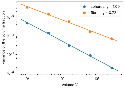
At the same volume the fraction of the fibres scatters far more, and the gap widens with the volume.
3. What a precision costs¶
rve_table turns a law into volumes: here the edge of the cube whose fraction is known
within 1 %, from one realization or as the mean of a hundred.
for name, fit in (("spheres", law), ("fibres", slow)):
    for row in rve.rve_table(fit, p, eps_rel=(0.01,), n=(1, 100)):
        print(name, row["n"], round(row["edge"]), f"{row['n'] * row['volume']:.2g}")
one realization |
100 realizations |
total volume, 1 then 100 |
|
|---|---|---|---|
spheres |
edge 93 |
edge 20 |
8.0·10⁵, 8.0·10⁵ |
fibres |
edge 559 |
edge 66 |
1.7·10⁸, 2.8·10⁷ |
Two lessons. The fibres ask for a cube six times as large as the spheres — two hundred
times their volume — for the same precision. And with γ = 1 a hundred small volumes
cost what one large volume costs, while with γ < 1 they cost less (six times less
here): long-range correlations make many small realizations the cheaper way, as long as
each is large enough for its boundary conditions not to bias its mean (compare the
means of the sizes; the periodic conditions bias least).
4. One large image: the window method¶
An image from a tomograph comes alone. Its non-overlapping windows stand for the
realizations: window_statistics gives the mean and the variance of the fraction over
windows of several edges (in voxels), shifts=2 adding the tilings shifted by half a
window on a periodic image.
large = spheres.generate(mg.Domain.cube(80.0, periodic=True), seed=3).voxelize(voxel_size=0.5)
windows = rve.window_statistics(large, [10, 16, 20, 32, 40], shifts=2)
print(windows.n)  # 4096, 1000, 512, 125 and 64 windows in one tiling
print(windows.volume * windows.variance / (p * (1 - p) * a3))  # 0.75, 0.86, 0.88, 0.96, 1.05
The variance of windows of 10 voxels — an edge of 5, two and a half diameters — is three
quarters of the asymptotic law: such windows are not yet large against the integral
range. Those of 32 voxels and more give the K of the theory within 5 %. A fit must
leave the small windows out (volume_range), or the volume it predicts is too small.
5. A physical property, from a configuration¶
The same statistics apply to every property that homogenize computes. A study is
described by a configuration with an rve section — the sizes, the realizations of
each, the properties — that morphogen run runs, in parallel (-j) or as the tasks of
a cluster (morphogen submit). Here the conductivity and the bulk modulus of the
spheres, a hundred times as conducting as their matrix, by the FFT solver:
from pathlib import Path

Path("rve.yaml").write_text(
    """
model: {type: boolean_spheres, radius: 1.0, volume_fraction: 0.16}
domain: {periodic: true}
seed: 1
voxels: {voxel_size: 0.5}
homogenization:
  method: fft
  materials:
    0: {young: 3.0, poisson: 0.35, conductivity: 0.2}     # a polymer: GPa, W/(m K)
    1: {young: 70.0, poisson: 0.22, conductivity: 20.0}   # a filler that conducts
  properties: [conductivity, bulk_modulus]
rve:
  sizes: [8.0, 12.0, 16.0]       # the edges of the cubes
  realizations: [32, 16, 8]      # of each size
  properties: [volume_fraction, conductivity, bulk_modulus]
  gamma: 1.0                     # imposed; without it the exponent is fitted too
  relative_errors: [0.01, 0.05]
  n_realizations: [1, 10]
outputs: {directory: out/rve, name: spheres}
""",
    encoding="utf-8",
)
morphogen run rve.yaml -j 4 # out/rve: results.csv, rve_report.md, .json, .tex, figures
From Python, the same run and its report:
import json

from morphogen import pipeline
from morphogen.config import load_config

outdir = Path(pipeline.run(load_config("rve.yaml")))
report = json.loads((outdir / "rve_report.json").read_text(encoding="utf-8"))
for name, series in report["properties"].items():
    first = series["rve"][0]  # the first precision asked: 1 %, one realization
    print(name, series["mean"], series["fit"]["K"], round(first["edge"]), first["edge_ci"])
property |
mean |
|
edge for 1 %, one realization |
|---|---|---|---|
volume fraction |
0.157 |
0.54 |
96 |
bulk modulus |
4.49 GPa |
55 |
48 |
conductivity |
0.52 W/(m K) |
15 |
131 |
The volume depends on the property: half the edge is enough for the bulk modulus, whose
contrast between the phases is moderate, and the conductivity — a contrast of 100 —
asks for more than the fraction itself. rve_report.md holds the tables of the method
(means and intervals of each size, bounds, isotropy of the mean tensors, the laws with
their confidence intervals, the volumes and the realizations needed) and the run writes
their figures, here the variance of the conductivity:
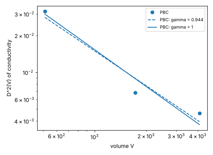
Three sizes and a few tens of realizations give K within a factor of two (the
interval of the edges above): a study to trust has more of both. The templates
rve_poisson_fibers, rve_multiphysics and rve_crystal_plasticity_fft of the
gallery are such studies, and rve_voronoi_windows one by the
window method.
Where next¶
The guide to the physics, §9: the names of the quantities that an
rvesection takes (a tensor, a result of a coupling, the stress or the strength of a loading path).The theory notes: the method and its estimators (§9), the statistics of apparent properties and the bias of the boundary conditions (§13).
morphogen fit results.csvfits the laws to a table of any origin;morphogen run study.yaml --resume,morphogen submitandmorphogen mergerun a long study in pieces (recipes).