Tutorial: a study in the graphical interface
The graphical interface runs the same functions as the Python snippets of the other
tutorials, from forms in the web browser: nothing to install besides morphoGen, nothing
sent anywhere (a local server on 127.0.0.1). This tour follows a small study — a
morphology, its measures, a loading path, a crack, its files — and shows where things
are. Each step takes a few seconds.
morphogen gui                 # opens http://127.0.0.1:8765/ in the browser
morphogen gui --port 9000 --no-browser
1. The page
The menus follow the work. Four sections in the header — Create, Characterize, Simulate, Export & compare — each with its tabs below; a tab lists its tools on its left, under the headings of what they do, with the form of the tool chosen beside them and its results on the right. Below the menus, the workspace keeps every morphology (M), simulation (S), behaviour of a material (B) and run of a tool (R) of the session: any tab takes its input from it, in any order.
In Create › Generate, the menu lists the 39 models by family (the filter above it
finds one by a word of its name or of its summary). Choose boolean_spheres: its form
opens filled with its template; set the radius to 1, the volume fraction to 0.2, the
size of the domain to 10 and the seed to 1, then Generate (or Ctrl + Enter, which
runs the form shown).
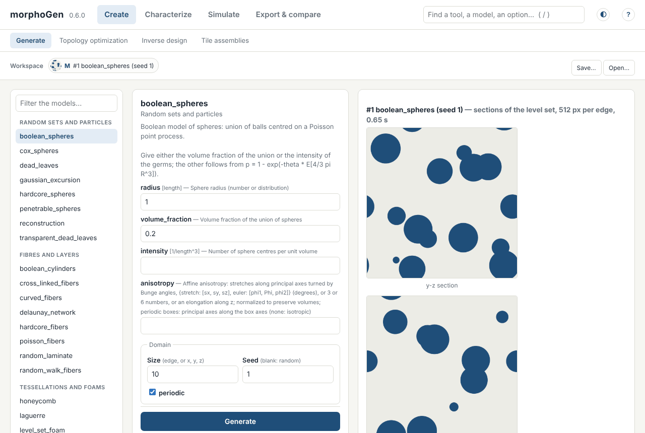
The page shows the sections of the realization (those of its implicit function,
computed at up to 2048 pixels per edge without a voxel image of the volume), a 3D view
that turns under the mouse, its measures against the theory of the model, and buttons
to send it on: Linear homogenization →, Statistics →, Export →. The morphology is
now the item #1 of the workspace.
2. Finding a tool or an option
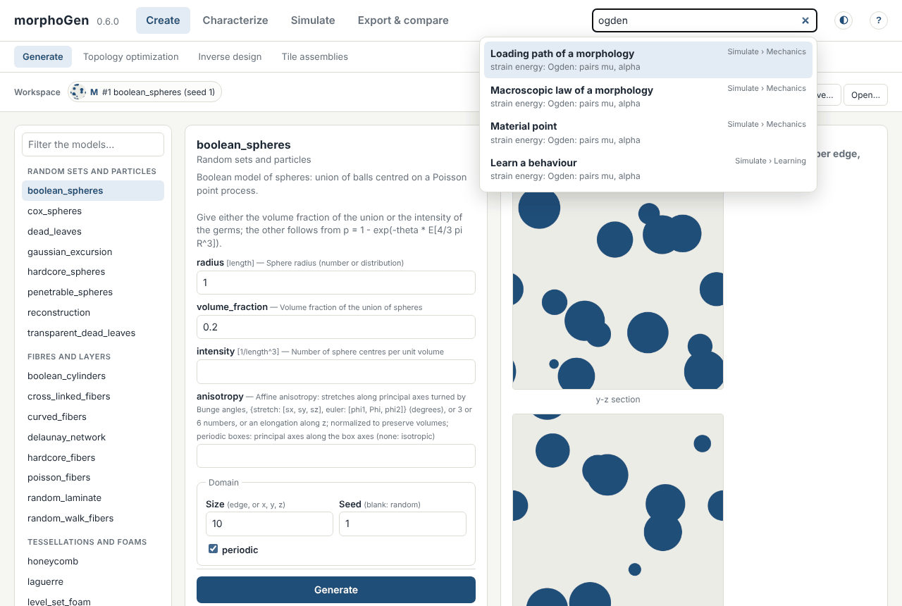
The search of the header (press /) looks through the tabs, the tools, the fields and
options of their forms, and the models, by the start of the words. It opens what it
finds with the option set: “ogden” opens the loading path of a morphology with the
hyperelastic behaviour and that strain energy chosen, “finite strains” its kinematics,
“stl” the surfaces of Export, “gyroid” the model of the triply periodic surfaces.
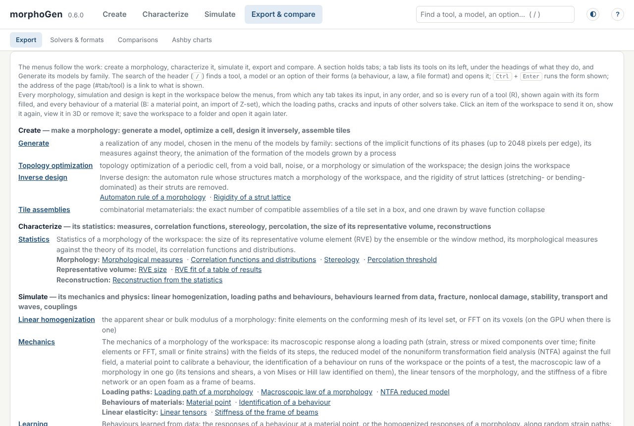
The address of the page names what is shown (#mechanics/path, #generate/voronoi):
a link to keep, or to give to a colleague who runs the interface. ? opens the map of
the interface, every tab and every tool as links:
3. Characterize
Statistics → below the sections sends the morphology to the tab Statistics, whose
first tool measures it on a voxel image: phase fractions, specific surface,
connectivity, chords, tortuosity… beside the closed forms of its model. The other
tools of the menu take the same morphology when they are chosen: its correlation
functions, its stereology, the percolation threshold of its model, the size of its
representative volume (by the ensemble or the window method), a reconstruction from its
statistics. The last tool of the menu, Orientation map (EBSD), starts from a file
instead: it finds the grains of an .ang or a .ctf map, draws its texture (the map in
the colours of its crystals, pole figures, the disorientations of its boundaries) and
adds its polycrystal to the workspace.
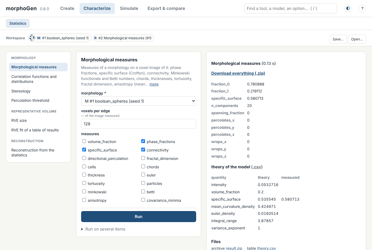
Each run joins the workspace (R): a click on its chip shows it again, its form filled with its parameters, to change them and run again.
4. Simulate
Simulate › Mechanics › Loading path of a morphology: the form stands in boxes — the morphology and the elastic constants of its phases, the behaviour of one of them (von Mises, crystal and porous plasticity, viscoelasticity, the hyperelastic energies, damage, a Z-set file, an MFront law, a behaviour of the workspace), the loading (a tension, a shear, cycles, or the components over time), the solver (FFT on voxels, or finite elements on a conforming mesh; small or finite strains). Two folded boxes go further: Interfaces (on the mesh, those of the phases or of the grains debond: a strength, a fracture energy, friction), Fatigue (a criterion and its two fatigue limits judge the points along the cycle: the utilization, the factor of safety) and Cleavage (the criterion of Beremin: the probability that the weakest point of the plastic zone has given way). With the defaults, the matrix yields under a tension to 1 %:
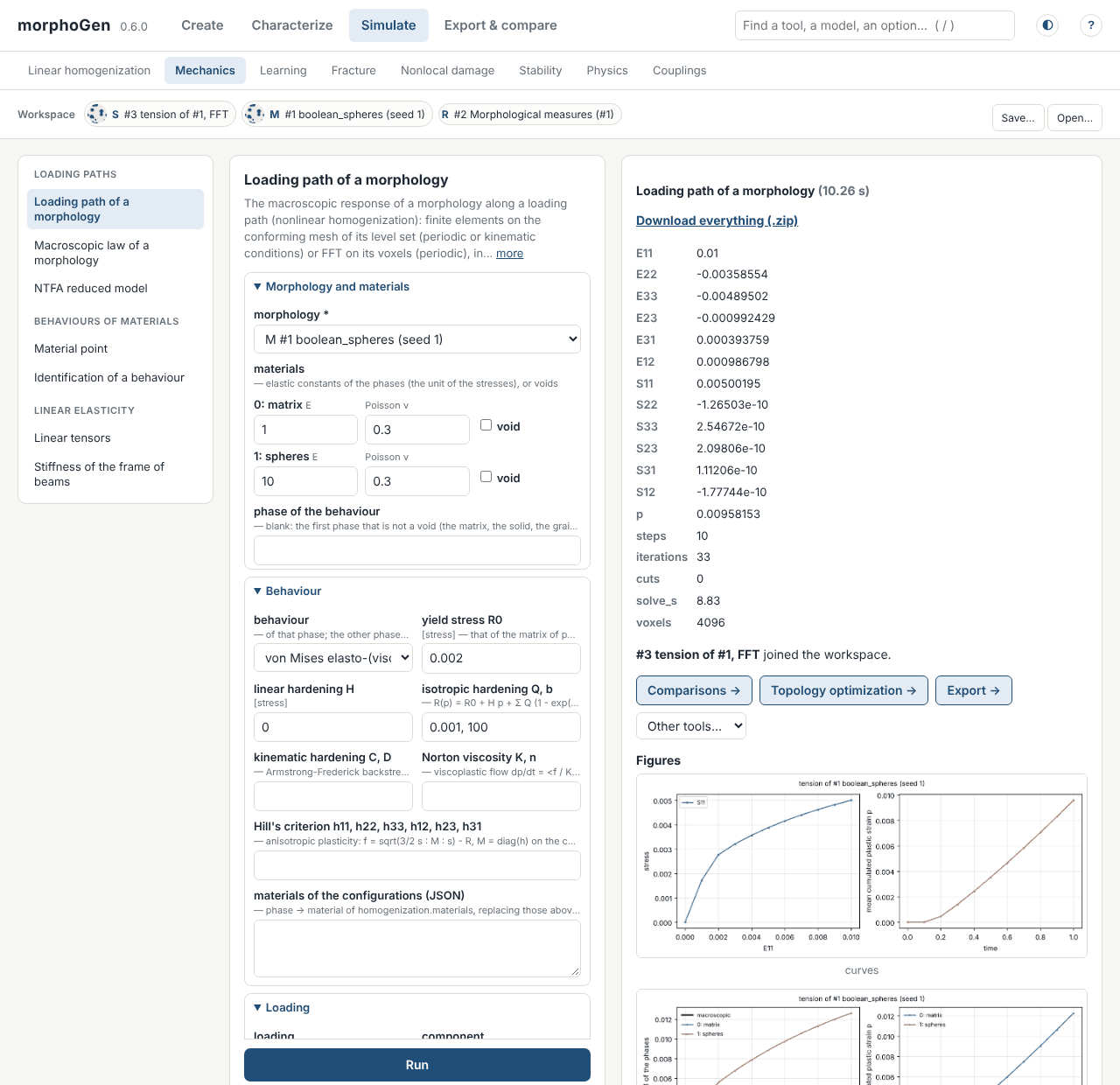
The result is a simulation (S) of the workspace, with its curves, its fields and the
configuration that runs it again with morphogen run. The other tabs of Simulate:
Linear homogenization (an apparent modulus with its fields), Learning (a
behaviour learned from responses), Fracture, Contact (a morphology between two
platens, or under an indenter), Nonlocal damage, Stability
(bifurcations, Bloch waves), Physics (transport, flow and sound, dynamic moduli,
band structures) and Couplings (diffusion, oxidation, hygromorphs).
5. Break it
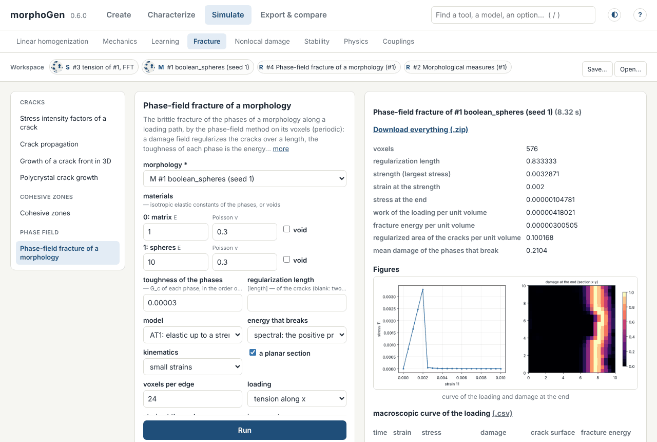
Simulate › Fracture › Phase-field fracture of a morphology pulls a planar section of the morphology until it breaks: the toughness of the phases that break, the regularization length (two voxels by default), the model (AT1, AT2), the energy that breaks, in small strains or, for rubbers, in finite strains. The matrix breaks at a strain of 0.2 %; the crack goes round the spheres, which have no toughness here and do not break.
A long computation is stopped by Stop beside its progress, at its next step.
6. Export
Export & compare › Export writes the files of an item with an archive of them all: of a morphology, its geometry (JSON), its sections, its implicit function and its voxel image (VTI), its surface (STL) and its conforming mesh (VTU) — for a morphology of several phases, the function and the surface of each phase —, and videos; of a simulation, figures, videos of its fields, tables and its configuration. Solvers & formats writes the inputs of AMITEX_FFTP and Abaqus, meshes and images for Gmsh, Neper, DAMASK…, the MFront sources of the behaviours; Comparisons draws the curves of several runs on one figure; Ashby charts the records of a database of results.
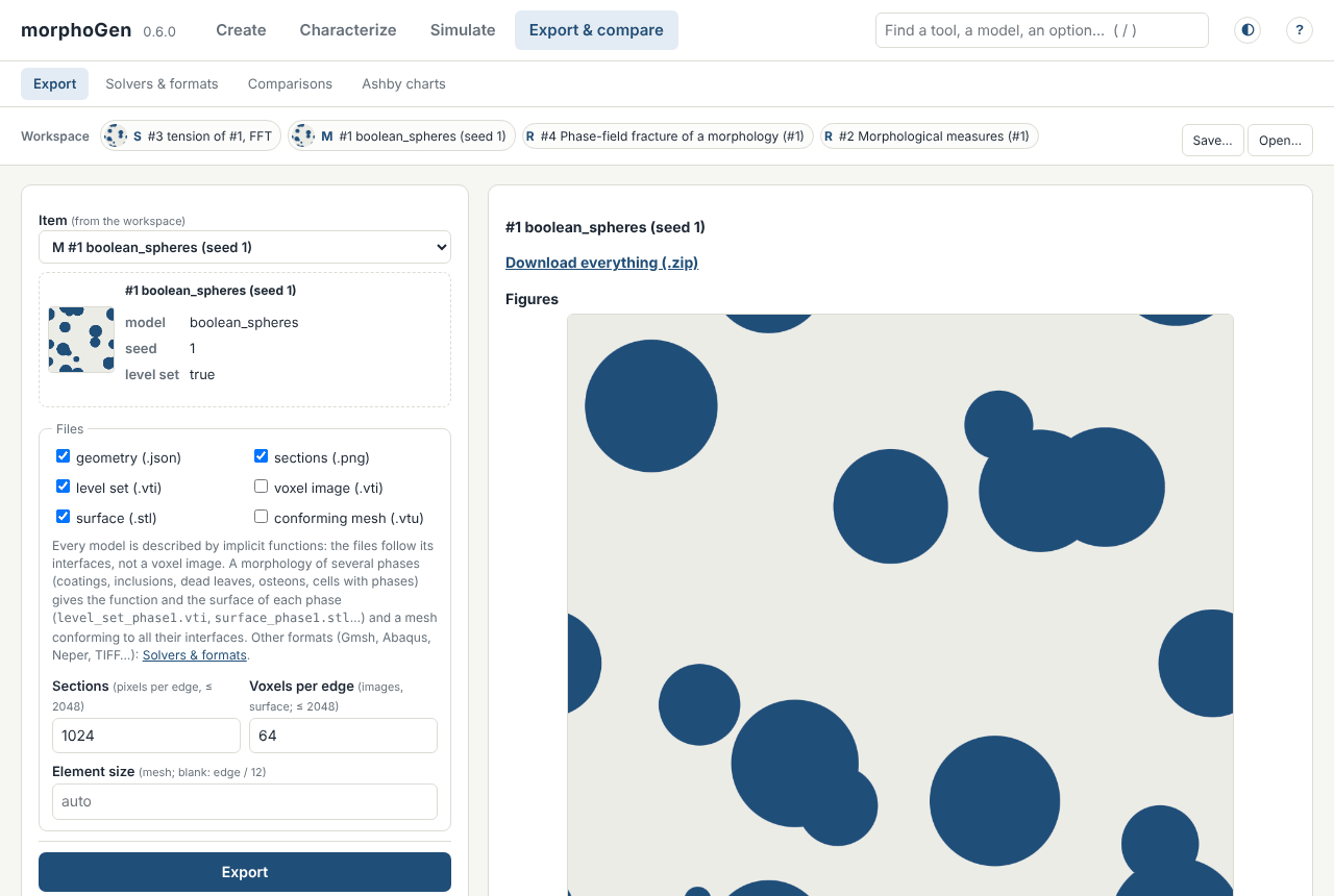
Save… beside the workspace writes it to a folder, Open… reads it back in another session.
Where next
The same study in Python: a whole study; the laws and the phase field of step 5 in finite strains: a rubber.
The graphical interface: every tab, tool by tool.
The screenshots of this page are taken by
python docs/tutorials/make_screenshots.py(Node.js and Playwright), which drives this very study in the page.